CS336 Note 02: PyTorch, Resource Counting

1. Memory accounting

1.1 tensor basics

tensor 是用来存储数据的基本单元：模型参数、梯度、优化器状态、激活状态等

1
2
3
4
x = torch.tensor([[1., 2, 3], [4, 5, 6]])
x = torch.zeros(4, 8) # 4x8 matrix of all zeros
x = torch.ones(4, 8) # 4x8 matrix of all ones
x = torch.randn(4, 8) # 4x8 matrix of iid Normal(0, 1) samples

也可以只分配内存但是不初始化值

1
x = torch.empty(4, 8)

1.2 tensor memory

几乎所有的数据都以浮点数的形式存储

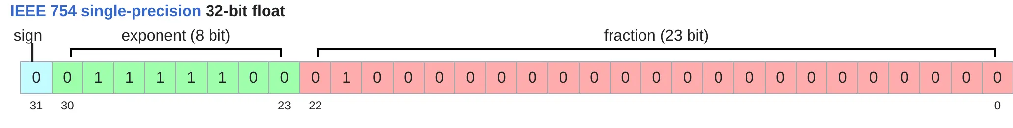
1.2.1 float32

在大多数情况下，float32 是默认的数据类型

数据的内存占用由数值的数量和数据类型决定

1
2
3
4
5
x = torch.zeros(4, 8)
assert x.dtype == torch.float32  # Default type
assert x.numel() == 4 * 8
assert x.element_size() == 4  # Float is 4 bytes
assert get_memory_usage(x) == 4 * 8 * 4  # 128 bytes

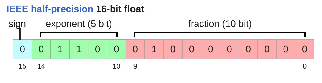
1.2.2 float16

float16 数据大小减半，但是可以表示的数值范围较小

1
2
3
4
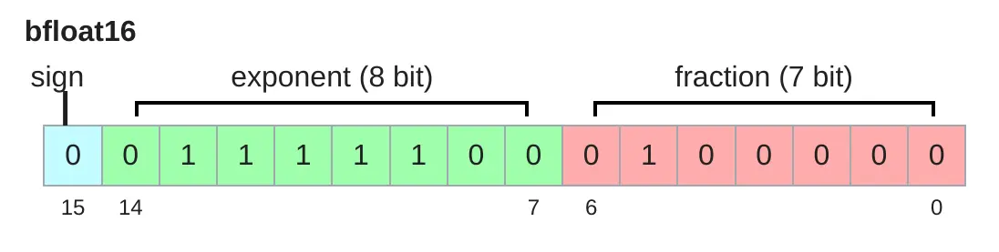
x = torch.zeros(4, 8, dtype=torch.float16)
assert x.element_size() == 2
x = torch.tensor([1e-8], dtype=torch.float16)
assert x == 0  # Underflow to 0

1.2.3 bfloat16

bfloat16 用来解决 float16 的动态范围问题，它和 float16 大小一致，但是有着和 float32 一样的动态范围，不过分辨率较差。对于深度学习来说动态范围比分辨率更重要

1
2
x = torch.tensor([1e-8], dtype=torch.bfloat16)
assert x != 0  # No underflow!

1.2.4 fp8

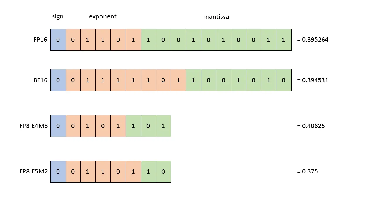
fp8 是另一种为机器学习设计的数据类型

使用float32 时训练效果较有效，但是需要较多的内存
使用 fp8、float16 和 bfloat16 可能导致训练存在风险，模型不稳定
一般可以使用混合精度训练

2. Compute accounting

2.1 tensor on gpus

默认 tensor 是存储在 CPU 上的，我们需要手动将其移动到 GPU

1
2
3
4
5
text("Move the tensor to GPU memory (device 0).")
y = x.to("cuda:0")
assert y.device == torch.device("cuda", 0)
text("Or create a tensor directly on the GPU:")
z = torch.zeros(32, 32, device="cuda:0")

2.2 tensor operations

2.2.1 tensor storage

在PyTorch 中，tensor 实际上是一个指向一块已划分内存的指针，是以 array 的形式存储，其中还包括了一些 metadata，告诉我们如何获取 tensor 的元素

1
2
3
4
5
6
x = torch.tensor([
	[0., 1, 2, 3],
	[4, 5, 6, 7],
	[8, 9, 10, 11],
	[12, 13, 14, 15],
])

1
2
3
4
5
6
7
assert x.stride(0) == 4  # 访问下方元素
assert x.stride(1) == 1  # 访问右侧元素

#　
r, c = 1, 2
index = r * x.stride(0) + c * x.stride(1)
assert index == 6

2.2.2 tensor slicing

很多对于 tensor 的操作只是返回了 tensor 的不同 view，并不是直接复制了一个 tensor，所以对 tensor 的修改互相影响

 1
 2
 3
 4
 5
 6
 7
 8
 9
10
11
12
13
14
15
16
x = torch.tensor([[1., 2, 3], [4, 5, 6]])

# 对tensor进行slicing
y = x[0]
assert torch.equal(y, torch.tensor([1., 2, 3]))
assert same_storage(x, y)

# 返回不同shape的view
y = x.view(3, 2)
assert torch.equal(y, torch.tensor([[1, 2], [3, 4], [5, 6]]))
assert same_storage(x, y)

# 转置
y = x.transpose(1, 0)  # @inspect y
assert torch.equal(y, torch.tensor([[1, 4], [2, 5], [3, 6]]))
assert same_storage(x, y)

有些操作会导致 tensor 变成 non-contiguous，导致后续无法再进行 view 操作。但是我们可以强制让 tensor 变成 contiguous

 1
 2
 3
 4
 5
 6
 7
 8
 9
10
11
12
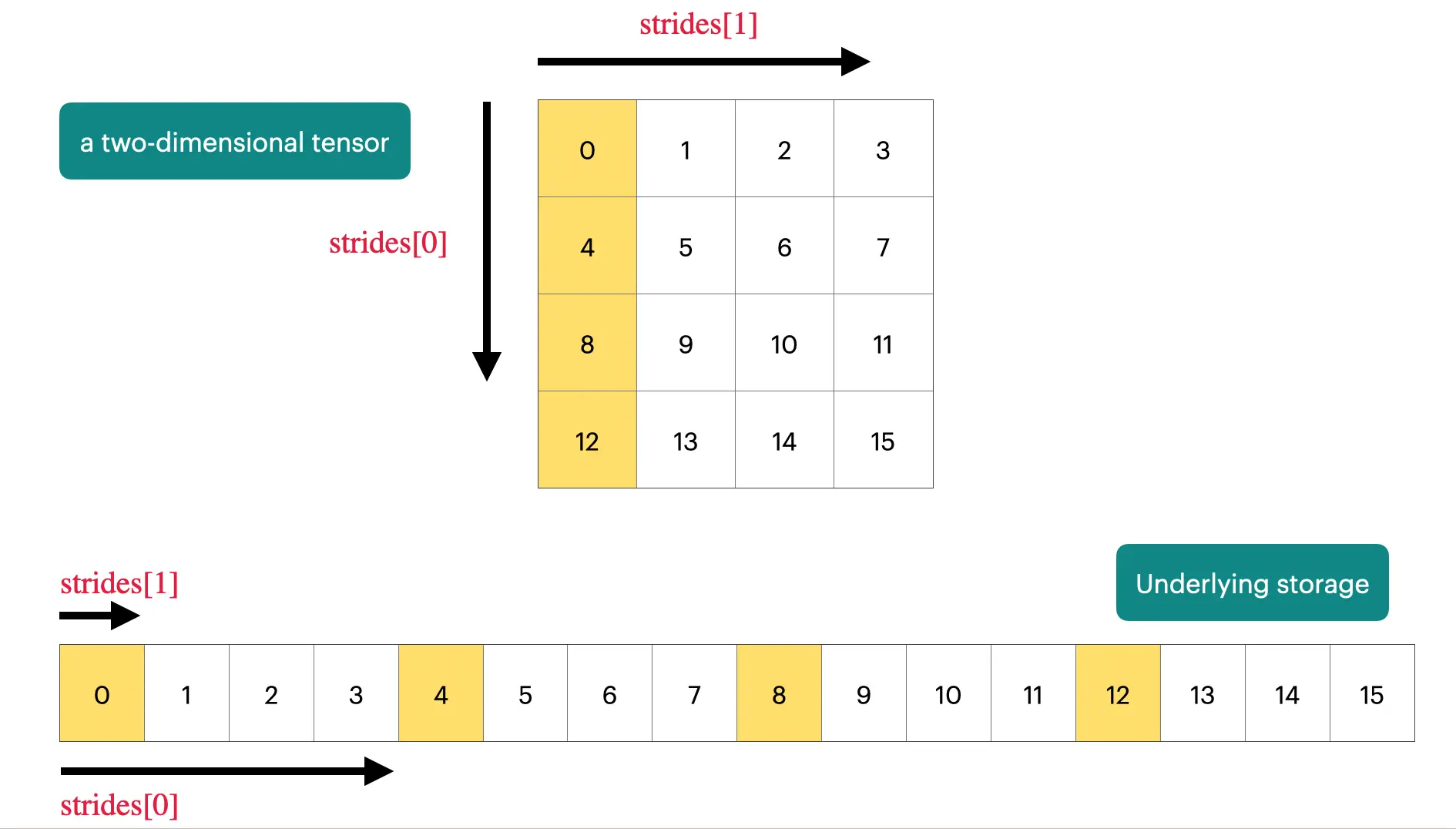
x = torch.tensor([[1., 2, 3], [4, 5, 6]])  # @inspect x
y = x.transpose(1, 0)  # @inspect y
assert not y.is_contiguous()
try:
	y.view(2, 3)
	assert False
except RuntimeError as e:
	assert "view size is not compatible with input tensor's size and stride" in str(e)

# 强制contiguous
y = x.transpose(1, 0).contiguous().view(2, 3)  # @inspect y
assert not same_storage(x, y)

2.2.3 tensor elementwise

elementwise 操作会对 tensor 的每个元素进行操作，并且返回一个形状相同的新 tensor

1
2
3
4
5
6
7
x = torch.tensor([1, 4, 9])
assert torch.equal(x.pow(2), torch.tensor([1, 16, 81]))
assert torch.equal(x.sqrt(), torch.tensor([1, 2, 3]))
assert torch.equal(x.rsqrt(), torch.tensor([1, 1 / 2, 1 / 3]))  # i -> 1/sqrt(x_i)
assert torch.equal(x + x, torch.tensor([2, 8, 18]))
assert torch.equal(x * 2, torch.tensor([2, 8, 18]))
assert torch.equal(x / 0.5, torch.tensor([2, 8, 18]))

2.2.4 tensor matmul

tensor 间也可以进行乘法运算，在多 batch 多 sequence 的情况下，乘法运算会 broadcast 到每一个token

1
2
3
4
x = torch.ones(4, 8, 16, 32)
w = torch.ones(32, 2)
y = x @ w
assert y.size() == torch.Size([4, 8, 16, 2])

2.3 tensor einops

einops 用来在操作 tensor 的时候，给每个维度命名

在 tensor 运算的时候，我们往往需要知道每个维度代表的意义。直接的方法我们可以通过注释标注，或者通过静态类型检查注明

1
2
x = torch.ones(2, 2, 1, 3) # batch seq heads hidden
x: Float[torch.Tensor, "batch seq heads hidden"] = torch.ones(2, 2, 1, 3)

einops 的 einsum 操作可以让维度标记更加方便

1
2
3
4
5
6
7
8
x: Float[torch.Tensor, "batch seq1 hidden"] = torch.ones(2, 3, 4)
y: Float[torch.Tensor, "batch seq2 hidden"] = torch.ones(2, 3, 4)

z = x @ y.transpose(-2, -1) # batch, sequence, sequence
# 等价于
z = einsum(x, y, "batch seq1 hidden, batch seq2 hidden -> batch seq1 seq2")
# 等价于
z = einsum(x, y, "... seq1 hidden, ... seq2 hidden -> ... seq1 seq2")

此外也支持维度收缩和 rearrange 操作

1
2
3
4
5
6
y = x.mean(dim=-1)
# 等价于
y = reduce(x, "... hidden -> ...", "sum")

x: Float[torch.Tensor, "batch seq total_hidden"] = torch.ones(2, 3, 8)
x = rearrange(x, "... (heads hidden1) -> ... heads hidden1", heads=2)

2.4 tensor operations flops

一个浮点运算（FLOP）是一个最基本的运算操作，例如加法和乘法

FLOPs：浮点运算的次数
FLOP/s：每秒浮点运算的次数

对于一个线性模型来说，如果有 B 个数据点，每个数据点是 D 维的，输出是 K 维的。输入数据 x 维度为 (B, D)，权值矩阵维度为 (D, K)，那么对于每个三元 index(i, j, k)，需要进行一次乘法运算 x[i][j] * w[j][k]，以及一个加法运算。总的 FLOPs 是 2 * B * D * K

前向传播中的 FLOPs 近似为 2 * 数据量 * 参数量

Model FLOPs utilization（MFU）：真实的 FLOP/s 除以额定 FLOP/s

2.5 gradients basics

PyTorch 中梯度计算非常简单，假定我们有一个线性模型 $y = 0.5 (x w - 5)^2$

1
2
3
4
5
6
7
x = torch.tensor([1., 2, 3])
w = torch.tensor([1., 1, 1], requires_grad=True)  # Want gradient
pred_y = x @ w
loss = 0.5 * (pred_y - 5).pow(2)

# 计算梯度
loss.backward()

2.6 gradients flops

假设有一个两层线性模型：h1 = x @ w1, h2 = h1 @ w2, loss = h2.pow(2).mean()

1
2
3
x = torch.ones(B, D, device=device)
w1 = torch.randn(D, D, device=device, requires_grad=True)
w2 = torch.randn(D, K, device=device, requires_grad=True)

对于参数矩阵 w2 来说

w2.grad[j, k] = sum_i h1[i, j] * h2.grad[i, j]，需要 FLOPs 2 * B * D * K
h1.grad[i, j] = sum_k w2[j, k] * h2.grad[i, k]，需要 FLOPs 2 * B * D * K

所以反向传播中 FLOPs 数量为 4 * 数据量 * 参数量

3. Models

3.1 module parameters

模型参数被保存在 nn.Parameter 对象中

对于 output = x @ w，x 经过 w 乘法之后，输出 output 的方差被放大 sqrt(input_dim)。导致输出的幅度变大，容易发生梯度消失。所以在初始化模型参数的时候往往会将方差缩小对应的倍数，这就是 Xavier 参数初始化

1
w = nn.Parameter(torch.randn(input_dim, output_dim) / np.sqrt(input_dim))

3.2 custom model

 1
 2
 3
 4
 5
 6
 7
 8
 9
10
11
12
13
14
15
16
17
18
19
20
21
22
23
24
25
26
27
28
29
30
class Linear(nn.Module):
    """Simple linear layer."""
    def __init__(self, input_dim: int, output_dim: int):
        super().__init__()
        self.weight = nn.Parameter(torch.randn(input_dim, output_dim) / np.sqrt(input_dim))

    def forward(self, x: torch.Tensor) -> torch.Tensor:
        return x @ self.weight

class Cruncher(nn.Module):
    def __init__(self, dim: int, num_layers: int):
        super().__init__()
        self.layers = nn.ModuleList([
            Linear(dim, dim)
            for i in range(num_layers)
        ])
        self.final = Linear(dim, 1)

    def forward(self, x: torch.Tensor) -> torch.Tensor:
        # Apply linear layers
        B, D = x.size()
        for layer in self.layers:
            x = layer(x)
        # Apply final head
        x = self.final(x)
        assert x.size() == torch.Size([B, 1])
        # Remove the last dimension
        x = x.squeeze(-1)
        assert x.size() == torch.Size([B])
        return x

默认 CPU tensor 被放置在 paged memory 中，我们可以手动 pin，这样就可以实现异步将 tensor 从 CPU 移动到GPU

1
2
3
if torch.cuda.is_available():
	x = x.pin_memory()
x = x.to(device, non_blocking=True)

3.3 randomness

为了实验结果可复现，一般需要设定固定的随机数种子

 1
 2
 3
 4
 5
 6
 7
 8
 9
10
11
# Torch
seed = 0
torch.manual_seed(seed)

# NumPy
import numpy as np
np.random.seed(seed)

# Python
import random
random.seed(seed)

3.4 data loading

在语言模型中，数据一般是一个 int 序列（字符 token 化的结果），我们可以很容易把它们作为 numpy array 序列化

1
2
orig_data = np.array([1, 2, 3, 4, 5, 6, 7, 8, 9, 10], dtype=np.int32)
orig_data.tofile("data.npy")

我们也可以从序列化数据文件中读取数据，通过 memmap 可以实现数据的懒加载，不把整个数据加载到内存中

1
data = np.memmap("data.npy", dtype=np.int32)

3.5 optimizer

几种常见的优化器

momentum = SGD + 梯度的指数移动平均
AdaGrad = SGD + 梯度平方的平均
RMSProp = AdaGrad + 梯度平方的指数移动平均
Adam = RMSProp + momentum

 1
 2
 3
 4
 5
 6
 7
 8
 9
10
11
12
13
14
optimizer = AdaGrad(model.parameters(), lr=0.01)

# 计算损失和梯度
x = torch.randn(B, D, device=get_device())
y = torch.tensor([4., 5.], device=get_device())
pred_y = model(x)
loss = F.mse_loss(input=pred_y, target=y)
loss.backward()

# 优化一步
optimizer.step()

# 清理内存
optimizer.zero_grad(set_to_none=True)

3.6 train loop

 1
 2
 3
 4
 5
 6
 7
 8
 9
10
11
12
13
14
15
16
17
18
19
20
def train(name: str, get_batch,
          D: int, num_layers: int,
          B: int, num_train_steps: int, lr: float):
    model = Cruncher(dim=D, num_layers=0).to(get_device())
    optimizer = SGD(model.parameters(), lr=0.01)

    for t in range(num_train_steps):
        # Get data
        x, y = get_batch(B=B)

        # Forward (compute loss)
        pred_y = model(x)
        loss = F.mse_loss(pred_y, y)

        # Backward (compute gradients)
        loss.backward()

        # Update parameters
        optimizer.step()
        optimizer.zero_grad(set_to_none=True)

3.7 checkpoint

训练模型往往需要非常长的时间，而我们不希望发生中断的时候遗失训练进度，所以在训练的过程中需要周期性的保存模型参数和优化器状态

 1
 2
 3
 4
 5
 6
 7
 8
 9
10
11
12
model = Cruncher(dim=64, num_layers=3).to(get_device())
optimizer = AdaGrad(model.parameters(), lr=0.01)

# 保存checkpoint
checkpoint = {
        "model": model.state_dict(),
        "optimizer": optimizer.state_dict(),
    }
torch.save(checkpoint, "model_checkpoint.pt")

# 加载checkpoint
loaded_checkpoint = torch.load("model_checkpoint.pt")

3.8 mixed precision training

数据类型（float32，bfloat16，fp8）的选择存在折衷

高精度：模型训练更加精准稳定，需要更多的内存和计算资源
低精度：模型训练不精准不稳定，需要更少的内存和计算资源

混合精度训练：默认使用 float32，但是在可行的地方尽可能使用 bfloat16 或者 fp8

在前向传播的时候使用低精度数据类型
在其他部分使用高精度数据类型（参数，梯度计算）