Transformer 的演变
Starting point: the original transformer
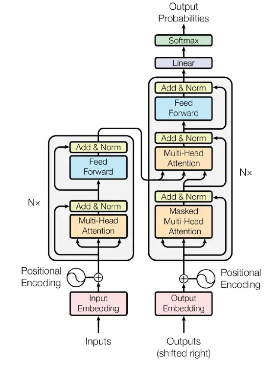
transformer
- Position embedding: sines and cosines
FFN: ReLU
$$FFN(x) = \max(0, x W_1 + b_1) W_2 + b_2$$Norm: post-norm, with LayerNorm
More simple and modern transformer variant
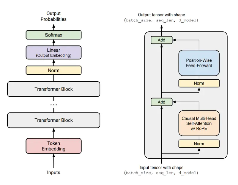
modern transformer variant
主要的不同:
- 使用了 pre-norm: LayerNorm 被放在了神经网络块和残差连接之前
- 使用了 Rotary position embedding (RoPE) 作为位置编码
- FFN 层被改造成 SwiGLU
- 线性层和 LayerNorm 不再使用偏置
Architecture
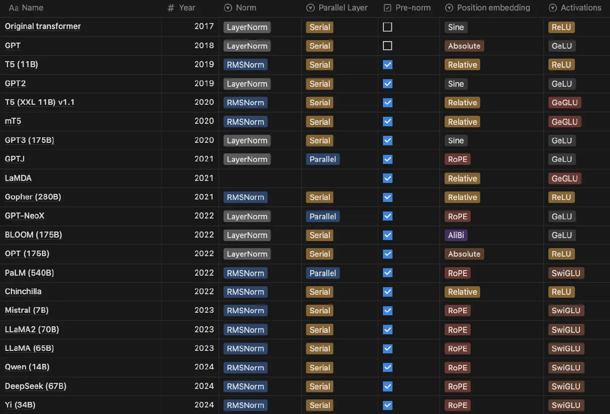
architecture of LLMs
Pre vs post norm
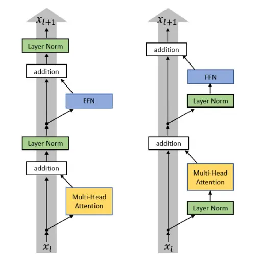
pre post norm
- post-norm
- pre-norm:LayerNorm 发生在 block 和残差之前,所以 Norm 不破坏残差连接的直接通路,更容易训练
几乎所有的现代 LM 都使用了 pre-norm (BERT 仍然使用 post-norm)
pre-norm advantages vs post-norm:
- original stated: 可以不使用 warmup
- today: 对于大型网络来说,训练更加稳定,可以使用更大的学习率
变种:double-norm
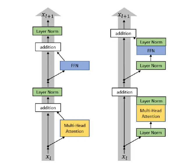
double norm
不太常见,在 Grok,Gemma 2 和 Olmo 2 中,只使用了 double-norm 的第二个 norm
LayerNorm vs RMSNorm
原始的 transfomer 使用了 LayerNorm,在 $d_{model}$ 的维度上,使用均值和方差归一化(GPT3/2/1,OPT,GPT-J,BLOOM)
$$y = \frac{x - \mathbb{E}[x]}{\sqrt{Var[x] + \epsilon}} \ast \gamma + \beta$$现代语言模型一般使用 RMSNorm,在归一化的时候不再考虑均值,并且去掉了偏置(LLaMa 系列,PaLM,Chinchilla,T5)
$$y = \frac{x}{\sqrt{\|x\|_2^2 + \epsilon}} \ast \gamma$$Why RMSNorm
- 比 LayerNorm 更快,但是表现也挺好
- 去掉了均值计算,更少的运算次数
- 去掉了偏置,更少的参数
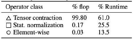
norm flops runtime
虽然 norm 的操作在总 FLOPs 中只占据非常小的比率(设计的矩阵运算较少),但是在运行时中却又较大影响(计算均值和方差,以及归一化,需要多次读写数据,所以 Norm 操作是内存密集型而不是计算密集型)
Activations
common activations:
ReLU: $ReLU(x) := max(0, x)$
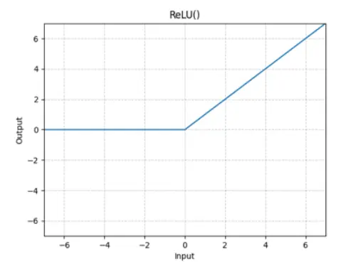
relu
used in original transformer, Google T5, Gopher, Chinchilla and OPT
GeLU: $GeLU(x) := x \Phi(x)$, where $\Phi(x)$ is the Cumulative Distribution Function for Gaussian Distribution
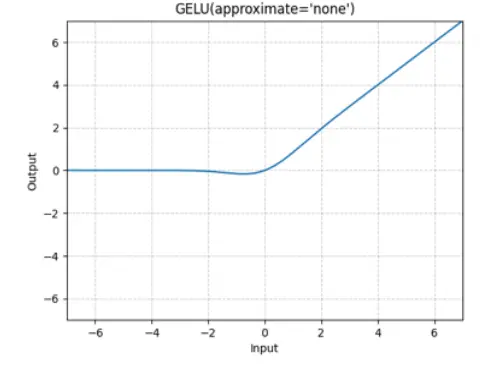
gelu
used in GPT1/2/3, GPT-Neox and BLOOM
There are also Gated activations (*GLU)
the original FF layer (without bias) is expressed as
$$FF(x) = max(0, xW_1)W_2$$In GLUs a FF layer is modified as
$$FFN(x) = (max(0, xW_1) \otimes (xV))W_2$$which is the linear + ReLU being augmented with an entrywise linear term
$$max(0, xW_1) \rightarrow max(0, xW_1) \otimes (xV)$$the Gated variants of FF layers:
GeGLU: $FFN_{GeGLU}(x) = (GeLU(xW_1) \otimes xV) W_2$
and SwiGLU (swish can be expressed as $Swish(x) = x \ast sigmoid(\beta x)$): $FFN_{SwiGLU}(x) = (Swish(xW_1) \otimes xV) W_2$
Some points about gating and activation:
- There are many variations (ReLU, GeLU and all kinds of GLU) across models
- GLU isn’t necessary but probably helpful
- Evidence points towards somewhat consistent gains from Swi/GeGLU
Serial vs Parallel layers
Normal transformer blocks are serial. They compute attention first, then the MLPs
$$y = x + MLP(LayerNorm(x + Attention(LayerNorm(x)))$$A few models (GPTJ, PaLM, GPT-NeoX) also do parallel layers
$$y = x + MLP(LayerNorm(x)) + Attention(LayerNorm(x))$$It’s stated that parallel ones result in faster training speed and roughly no quality degradation at large scales
Position Embedding
Many variations in position embeddings
Sine embeddings: add sines and cosines that enable localization (used in original transformer)
$$ \begin{gathered} Embed(x, i) = v_x + PE_{pos, i} \\ PE_{pos, i} = \sin(pos / 10000^{2i / d_{model}}) \\ PE_{pos, 2i + 1} = \cos(pos / 10000^{2i / d_{model}}) \end{gathered} $$Absolute embeddings: add a position vector (learnable) to the embedding (used in GPT1/2/3 and OPT)
$$Embed(x, i) = v_x + u_i$$Relative embeddings: add a relative position vector to the attention computation (used in Google T5, Gopher and Chinchilla)
$$e_{ij} = \frac{x_i W^Q (x_j W^K + a_{ij}^K)^T}{\sqrt{d}}$$RoPE: rotary position embeddings
the one that used most widely in LLM
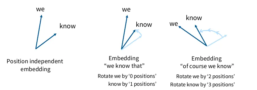
A high level thought
when we get a positional embedded vector $f(x, i)$,we want it to work like
$$\left< f(x, i), f(x, j) \right> = g(x, y, i - j)$$That is, in attention, the output of two positional embedded vectors $g(x, y, i - j)$ only gets to depend on the relative positon $(i - j)$.
But most of the existing embeddings not fulfill this goal
Sine: There are various cross-terms that are not relative (Taylor expansion)
$$\left< Embed(x, i), Embed(y, j)\right> = \left< v_x, v_y \right> + \left< PE_i, v_y \right> \cdots$$Absolute: obviously not relative
Relative embeddings: $e_{ij} = \frac{x_i W^Q (x_j W^K + a_{ij}^K)^T}{\sqrt{d}}$ is not an inner product format
We know that inner products are invariant to arbitrary rotation. Whatever rotation we apply, the inner product of two vectors remains unchanged
So we apply different rotation on two vectors based on their position. Then, the inner product of these two only depends on their relative position, but not the absolute position of each vector. (As illustrated below)
rotation
How to apply rotary position embedding
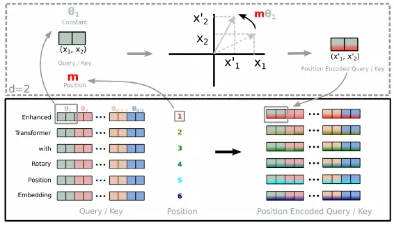
rope draw
将 vector 在特征维度上两两打包成一个复数,在复平面上,施加于当前 vector 的位置和 index on dimension 有关的旋转矩阵 $\begin{pmatrix} \cos m\theta & -\sin m\theta \\ \sin m\theta & \cos m\theta \end{pmatrix}$,之后再将旋转后的复数拆分成两个实数值,重新组合成 vector
这个过程其实就是将 vector 乘了一个 rope 矩阵
$$f_{\{q, k\}} (\mathbf{x}_m , m) = \mathbf{R}_{\Theta, m}^d \mathbf{W}_{\{q,k\}} \mathbf{x}_m$$这个矩阵可以表示为
$$ \mathbf{R}_{\Theta, m}^d = \begin{pmatrix} \cos m\theta_1 & -\sin m\theta_1 & 0 & 0 & \cdots & 0 & 0 \\ \sin m\theta_1 & \cos m\theta_1 & 0 & 0 & \cdots & 0 & 0 \\ 0 & 0 & \cos m\theta_2 & -\sin m \theta_2 & \cdots & 0 & 0 \\ 0 & 0 & \sin m\theta_2 & \cos m \theta_2 & \cdots & 0 & 0 \\ \vdots & \vdots & \vdots & \vdots & \vdots & \vdots & \vdots \\ 0 & 0 & 0 & 0 & \cdots & \cos m\theta_{d / 2} & -\sin m\theta_{d / 2} \\ 0 & 0 & 0 & 0 & \cdots & \sin m\theta_{d / 2} & \cos m\theta_{d / 2} \end{pmatrix} $$Hyperparameters
FFN: model dimension ratio
the relationship between the feedforward dim $d_{ff}$ and the model dim $d_{model}$
at most cases, there is a convention
$$d_{ff} = 4 d_{model}$$特例1 - GLU
在原始的 FFN 中,主要有两个权值矩阵 $W_1, W_2$,参数量为 $2 d_{model} d_{ff}$,如果取 $d_{ff} = 4 d_{model}$,那么参数量就是 $8d_{model}^2$
在 SwiGLU 中,除了 $W_1, W_2$ 之外,还有一个值矩阵 $V$,总参数量为 $2 d_{model}d_{ff}' + d_{model} d_{ff}'$,为了让参数量仍然为 $8 d_{model}^2$,此时 $d_{ff}' = \frac{8}{3} d_{model}$
特例2 - T5
$d_{ff} = 65536, d_{model} = 1024$
Head-dim*num-heads to model-dim ratio
在大多数模型里面 head-dim = model-dim / num-heads,但是也有一些模型设置 head-dim > model-dim / num-heads
Deeper or wider
大多数模型 $d_{model} / n_{layer}$ 处于一个固定范围内
| model | $d_{model} / n_{layer}$ |
|---|---|
| BLOOM | 205 |
| T5 v1.1 | 171 |
| PaLM(540B) | 156 |
| GPT3 /OPT/Mistral/Qwen | 128 |
| LLaMa/LLaMa2/Chinchila | 102 |
| T5(11B) | 43 |
| GPT2 | 33 |
如果模型太深,难以并行化,推理时延更高
Vocabulary size
单语言模型 30-50K
多语言模型 100-250K
Dropout and regularization
大多数模型都会在预训练中使用 dropout,最近的一些模型倾向于只使用 weight decay 而放弃了 dropout
Stability
softmax 存在计算级数,以及除以 0 的操作,容易造成训练不稳定
在 softmax 中
$$ \begin{gathered} \begin{align*} \log (P(x)) & = \log \left( \frac{e^{U_r(x)}}{Z(x)} \right) \\ & = U_r(x) - \log(Z(x)) \end{align*} \\ Z(x) = \sum_{r' = 1}^{|V|} e^{U_{r'}(x)} \end{gathered} $$由于存在 $\exp(\cdot)$ 操作,如果某些输出的 logit $U_{R}(x)$ 过大, $Z(x)$ 就会过大,可能存在数值溢出
z-loss,在原本的损失的基础上,添加一个关于 $Z$ 的惩罚项,让它不要过大。虽然 logit 的数值大小受到了惩罚约束,但是只要 logit 之间的相对大小不变,softmax 的结果保持不变
$$ \begin{align*} L & = -\sum_i [\log(P(x_i)) \textcolor{red}{- \alpha (\log (Z(x_i)) - 0)^2}] \\ & = \sum_i [-\log (P(x_i)) \textcolor{red}{+ \alpha \log^2 (Z(x_i))}] \end{align*} $$在上式中 $\alpha \log^2 (Z(x_i))$ 需要尽可能小,所以 $Z(x_i)$ 尽可能接近 1,被限制在合理的范围内
soft-capping,限定 logit 的值在 -soft_cap 和 +soft_cap 之间,可以通过 tanh 激活函数实现
$$logits \leftarrow soft\_cap \ast tanh(logits / soft\_cap)$$这种方法似乎会导致性能下降
Attention heads
多头注意力主要有两种变体
- GQA/MQA:通过减少头数提高推理效率
- Sparse or slideing window attention:限制注意力的模式来降低计算开销
GQA and MQA
在训练和 Prefill 阶段,所有的 token 是同时并行计算的,此时是计算密集型
总计算量为 $O(bnd^2)$,内存访问量为 $O(\underbrace{bnd}_{x} + \underbrace{bhn^2}_{softmax} + \underbrace{d^2}_{projection})$
此时 Arithmetic intensity (计算量/内存访问量)为 $O\left( \left( \frac{1}{k} + \frac{1}{bn}\right)^{-1} \right)$,GPU 的利用率较高
在生成阶段,无法使用并行计算,往往会采用 KV Cache 的方法,把之前计算过的 Key 和 Value 保存下来。这时每次新生成 token 时,我们会去读取过去所有 token 的 KV Cache,每次的计算量比较小,但是内存访问量非常大,变成了访问密集型,GPU 利用率不高
所以我们需要降低 KV Cache 的内存访问量
通过 GQA 和 MQA 可以减少需要存储的 KV Cache
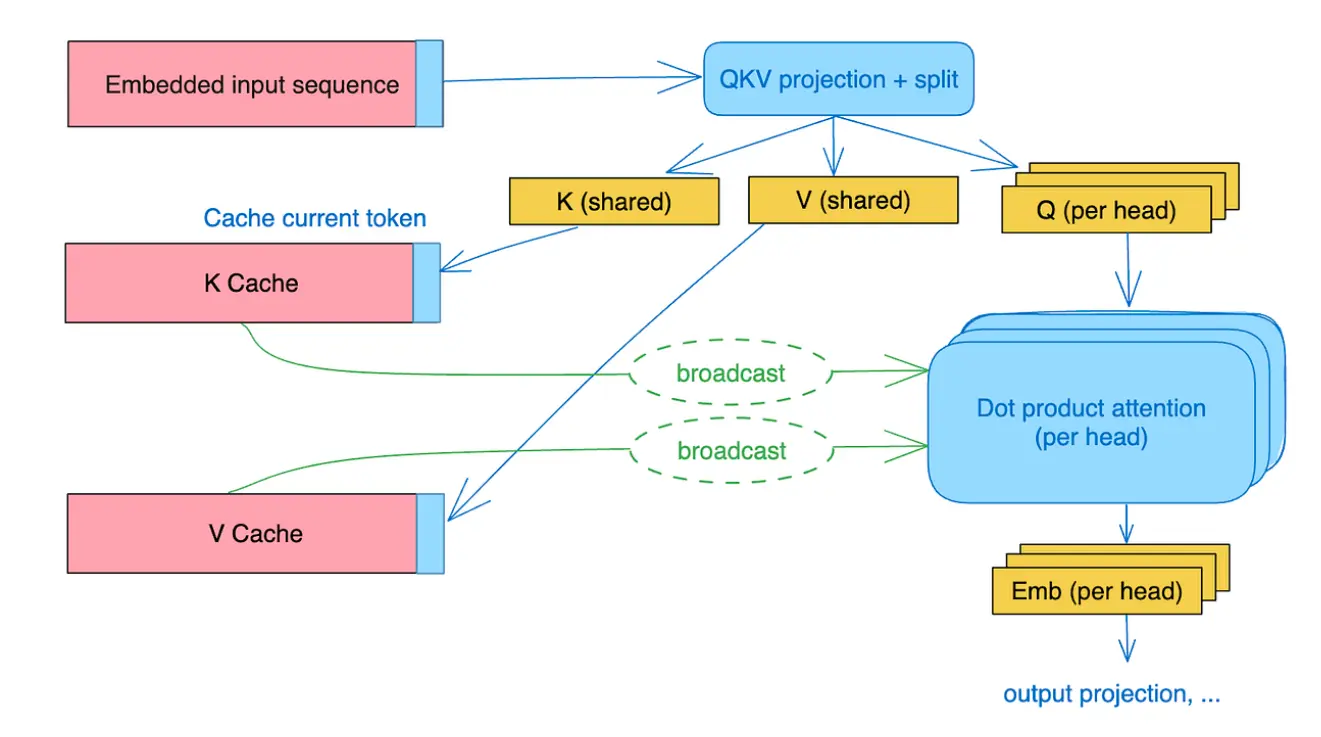
mqa
在 MQA 中,每个 query 共享同一个 key 和 value
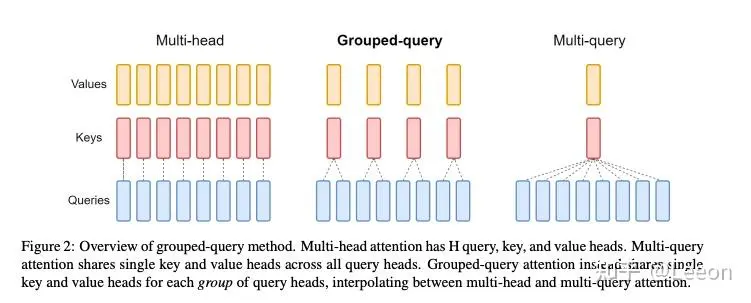
mqa and gqa
在 GQA 中则是一组内的 query 共享同一个 key 和 value
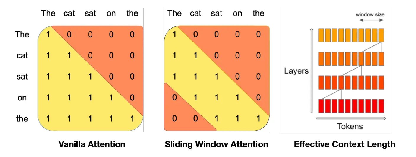
Sparse/sliding window attention
对整个上下文使用注意力计算开销较大,所以演变出了 sparse 和 sliding attention
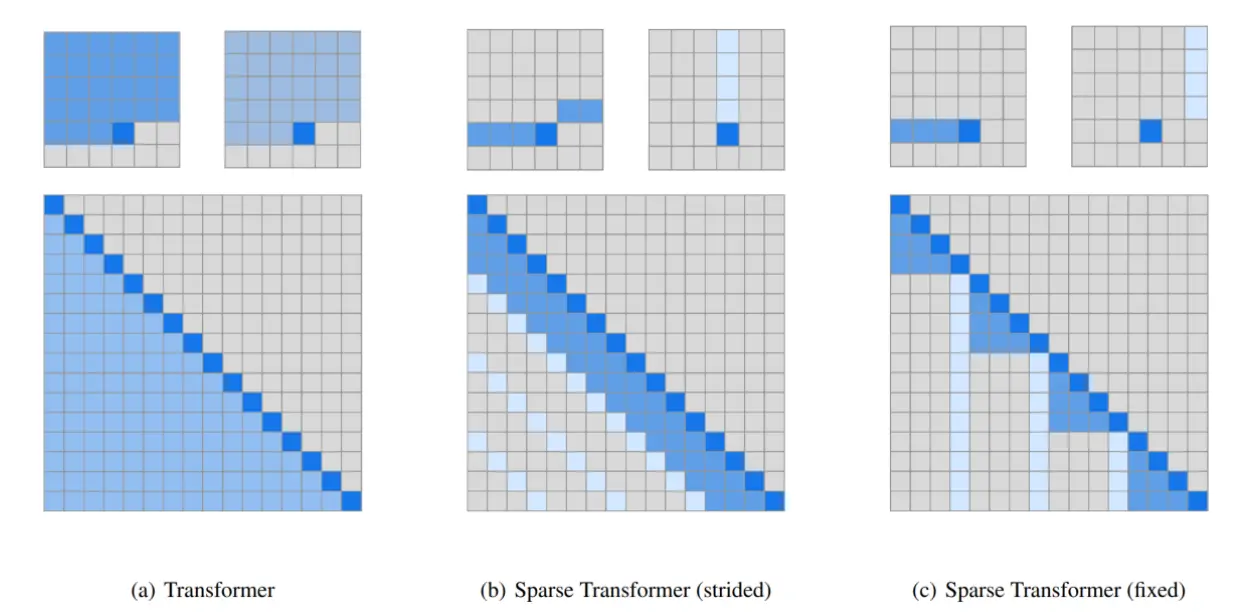
spare attention